Building an IFRS 17 GMM forecast: the projection mechanics

FY2026 is the first full budget cycle most life insurers, long-tail non-life writers, and reinsurers are running on IFRS 17 GMM baselines. The mechanics are different again from PAA — earned premium is replaced by a build-up of CSM release, RA release, expected claims and expenses, and NDAC amortisation; the balance sheet carries a contractual service margin or a loss component instead of UPR and DAC; locked-in and current discount rates coexist; and every future period is a fresh bottom-up valuation of each cohort.

For the teams building these forecasts — and the heads of actuarial, group reporting, and audit committees consuming them — the risk is a forecast that reconciles against IFRS 4 or PAA habits but misstates the IFRS 17 result. The sections below set out how the projection is built, and the mechanics that are specific to GMM.

This post walks through how the projection is built, the views it should produce, and the nuances behind each. It is the second post in the forecasting series — the PAA version was released in April — and this one is built from a working GMM demo with realistic data, full projections, and scenario analysis.

What a forecast actually does

A forecast projects your insurance result forward, period by period, under a set of assumptions. Under GMM it lets you test scenarios, gauge combined-ratio trajectories, plan capital coverage, and design pricing or reinsurance changes that re-establish a CSM on cohorts heading onerous. A GMM forecast that does only the first two of those is of limited use. One that does all five supports the decisions a forecast exists for.

How a GMM forecast is built

Three pieces.

Inputs. The closing in-force position at the latest valuation date, per IFRS 17 group: BEL fulfilment cash flows over future periods, CSM balance and the coverage units attaching to each future period, locked-in discount rates from initial recognition, RA balance, Loss Component where the group is onerous, plus the reinsurance mirror. Alongside that, the latest-year new business initial-recognition run — the template from which future cohorts are layered.

Mechanic. At each future period, every active cohort is rolled forward by a present-value recursion. The BEL unwinds at current rates. The CSM unwinds on its own locked-in curve and releases on coverage units. Where a group carries an LC instead, the LC reduces by systematic allocation as the claims, expenses and RA it covers release from the LFRC. The RA — a load on claims and expenses, a flat 5% in this demo and calibrated to a stated confidence level (a scenario-test or cost-of-capital basis) in production — releases as the risk emerges. A new cohort is written and recognised from first principles: at initial recognition a profitable group’s CSM is the present value of inflows less outflows, less the RA and acquisition costs (paragraph 38), and where that figure is negative the group is onerous — instead of a negative CSM the day-1 loss goes to the P&L with a loss component set up against it. The result is summed across cohorts.

New-business volumes are an explicit assumption. Approaches are emerging that leverage the latest new business year and scale each cash-flow type into the future on its own factor — premium growth separate from claims and expense factors, calibrated to how you expect experience to differ in future periods. Variable expenses grow with the book; overheads grow at a pace different to the premium growth assumptions.

Modelling the income statement into the future is not as simple as projecting income statement line items forward. To project adequately, the balance sheet is projected, and the movements in its components — BEL, RA, CSM, LIC BEL and RA — flow into the P&L. That is what determines how the reserves run off and how insurance finance income and expense behave in future periods. The same care applies on the balance-sheet side: debtors and creditors need explicit assumptions for how they grow and run off over time, and the LIC has its own dynamic: it increases with newly incurred claims, which raise the OCR and IBNR via current service movements, and runs off as claims are reported and settled via past service — with the run-off needing assumptions for how those components develop. That balance drives how the LIC grows or reduces over time, which in turn drives how its unwind and RA grow or reduce.

Output. Projected SOCI lines built from the IFRS 17 revenue components (CSM release, RA release, expected insurance service expenses, NDAC amortisation, premium experience variance), balance-sheet roll-forwards per IFRS 17 group, plus the cash leg — premium debtors, expense and acquisition creditors, claims paid to bank — and the bank trajectory.

Asking the client for the inputs — three options

Three viable input paths exist; the first conversation is which one the client’s systems can produce.

Option A — pre-discounted PV cash flows. The client supplies fully-discounted PVs per group, decomposed by Analysis-of-Movements walk. Client owns discounting. Suitable for clients with a mature internal discounting engine. Client effort highest, our effort lowest.

Option B — undiscounted cash flows at IFRS 17 group level. Recommended production path for most mid-sized insurers. The client supplies undiscounted cash flows per group per future year, by cash-flow type. We apply discounting, RA, and the CSM and LC machinery. Client effort moderate; our effort moderate; audit reproducibility high. This is what Prophet, AXIS, ResQ, MoSes and similar reserving systems export natively.

Option C — per-policy / model point file. Row-per-policy file. We project the cash flows from scratch per policy per month, aggregate to groups, then discount. Heaviest path on our side; ideal for prototyping or scenario design. Not a recommended production path because most clients prefer not to share policy-level data with external actuaries, and the model is harder to validate at the IFRS 17 group level — which is where the auditor signs.

---

Four mechanics GMM requires that PAA does not

Before the views, a quick orientation. These four mechanics are explicit in GMM measurement and absent or only implicit under PAA, so a forecast has to model each one directly.

Locked-in vs current rates. The CSM unwinds on the locked-in curve set at initial recognition of each cohort (IFRS 17 paragraph B72). The BEL, RA, and LC roll forward on the current curve as at each reporting date (paragraph 36). The forecast preserves both rate vectors per cohort. Locked-in is locked-in for the CSM accretion rate only — it is not locked-in for the BEL. An easy detail to get wrong. The curve itself is flat in this demo (a single rate across maturities); a production forecast sources a term structure — the sovereign zero-coupon curve plus an illiquidity premium calibrated to the portfolio.

Coverage-unit CSM release. The CSM releases as the coverage units attaching to the current period divided by the total remaining coverage units (paragraph B119) — a basis chosen deliberately, in practice often proxied by earned premium (as this demo does) or by an expected-coverage measure. A twelve-month Property contract releases its CSM faster than an eighty-four-month Casualty contract over the same calendar period.

Layering future new business. At any future date, several cohorts are simultaneously on the balance sheet at different ages: the in-force, plus the cohort written in year 1 at age t-1, plus year 2 at t-2, and so on. Treating new business as a single growth scalar on the in-force collapses that layering and materially understates the diversity of cohorts you actually carry.

Onerous recognition and the CSM-to-LC boundary. An IFRS 17 group carries either a CSM or a Loss Component — never both. The determination is made at each cohort’s initial recognition: a cohort whose combined ratio exceeds 100% on a discounted basis is onerous, books its day-1 loss to the P&L and sets up an LC. This is not only a stress phenomenon — a base forecast routinely carries some onerous cohorts (a thinly-priced underwriting year is onerous in the central case), so the loss-component machinery is exercised in the base run, not just under shock. What a base forecast generally does not do is switch a group mid-life: future-service assumption updates on in-force groups are typically not modelled, so a profitable group does not flip to onerous between valuation dates. Scenario analysis is where the boundary moves the most — a shocked future cohort lands onerous at its own initial recognition, and the model has to detect which side of zero each group falls on and post accordingly.

One more GMM-specific point: the actuals live inside the balance-sheet measurement. Receivables and payables that sit outside the measurement under PAA are inside it here, so a difference between actual raised and model-expected raised on unearned premium triggers a CSM unlock — the debtor and creditor assumptions reach the P&L, not just the bank position.

---

New business layering per portfolio — one growth rate misses the future-state mix

A common simplification is one growth rate across the book. It collapses that layering.

In practice, per-portfolio trajectories diverge. The volume scalars below are illustrative — actual values come from a business plan, market data, and recent experience — but the shape of the disagreement is structural.

Portfolio	Annual scalar	Story
Property	×0.95	Improving book, declining volume; tighter underwriting
Casualty	×1.08	Growing exposure; expanding lines, longer-tail mix
Engineering	×1.15	Cycle-sensitive expansion; project pipeline driving growth
Marine	×1.00	Mature and stable; volume flat, claims discipline doing the work

Layered cohort by cohort over five years, Engineering compounds to roughly twice its starting weight while Property falls below 0.8 of its current scale. The mix at year five is a different book to the one in force today. A forecast that scales all four at, say, ×1.05 produces a fictional future-state mix.

Per-cash-flow-type scalars are a further refinement — where pricing is repositioning, premium can be scaled differently to claims for future cohorts.

---

Scenario analysis — four scenarios on the same book

The demo projects the same book under four scenarios: BASE, a uniform claims stress (loss ratios × 1.10), an expense squeeze (expense ratios × 1.10), and the Catastrophe Shock 2027 described below. The stresses are multiplicative overlays on BASE, so the per-portfolio storylines — Property improving, Casualty deteriorating, Engineering cycle-sensitive, Marine stable — stay visible in every scenario. In the central case the book runs around an 85% combined ratio; the uniform stresses lift the total a few points, while the catastrophe concentrates a 130–150% combined in the 2027 cohort alone.

The purpose is to compare the impact on the balance sheet and the P&L side by side: insurance result per period, BEL closing, combined ratio, and CSM closing balance across all four scenarios on one set of axes. A uniform stress moves every cohort; the discrete shock concentrates in the 2027 cohort with a partial 2028 recovery. Seeing both in the same view is what makes the comparison useful.

The Catastrophe Shock 2027 scenario — how a discrete cohort shock lands

A discrete-shock scenario exercises mechanics that uniform stress does not. The shape: a single-year event in 2027 pushes claims up 30% and expenses up 10% in the 2027 cohort. Recovery is partial in 2028 (claims +15%, expenses +5%). From 2029 the book is back to BASE. Other cohorts unaffected.

Under GMM this is a multi-cohort story. The 2027 cohort, with a combined ratio between 130% and 150%, is onerous at initial recognition. A Loss Component is established at sale; the loss is booked to P&L in 2027. Reinsurance damps the net effect — the loss-recovery component on the ceded balance picks up the reinsurer’s share, computed as r = expected RI recoveries / total underlying claims applied to the covered portion of the LC. For a vanilla proportional cover, r collapses to the ceding ratio. For excess-of-loss or aggregate stop-loss, r depends on the shape of the underlying claims distribution.

The 2028 cohort, written at +15% loss and +5% expense, may or may not be onerous depending on baseline margin — a smaller LC if so, a smaller CSM if not. From 2029, cohorts behave as if nothing happened — the shock is discrete rather than a regime change.

What the scenario tests:

1. The shocked 2027 cohort books its day-1 loss in the right year, in the right group, with the right residual.
2. The LC release in subsequent periods shadows the BEL runoff of the shocked cohort, not the book at large.
3. The reinsurance loss-recovery component is calculated on the LC, not on underlying claims volume.
4. 2029 returns to a clean BASE without bleed-through from the 2027/28 onerous tail.

Both belong in the scenario set.

---

View 1 — Implied vs assumed assumptions, with CSM release alongside

A useful starting point. Under GMM the comparison is richer than PAA’s loss-ratio-vs-assumed.

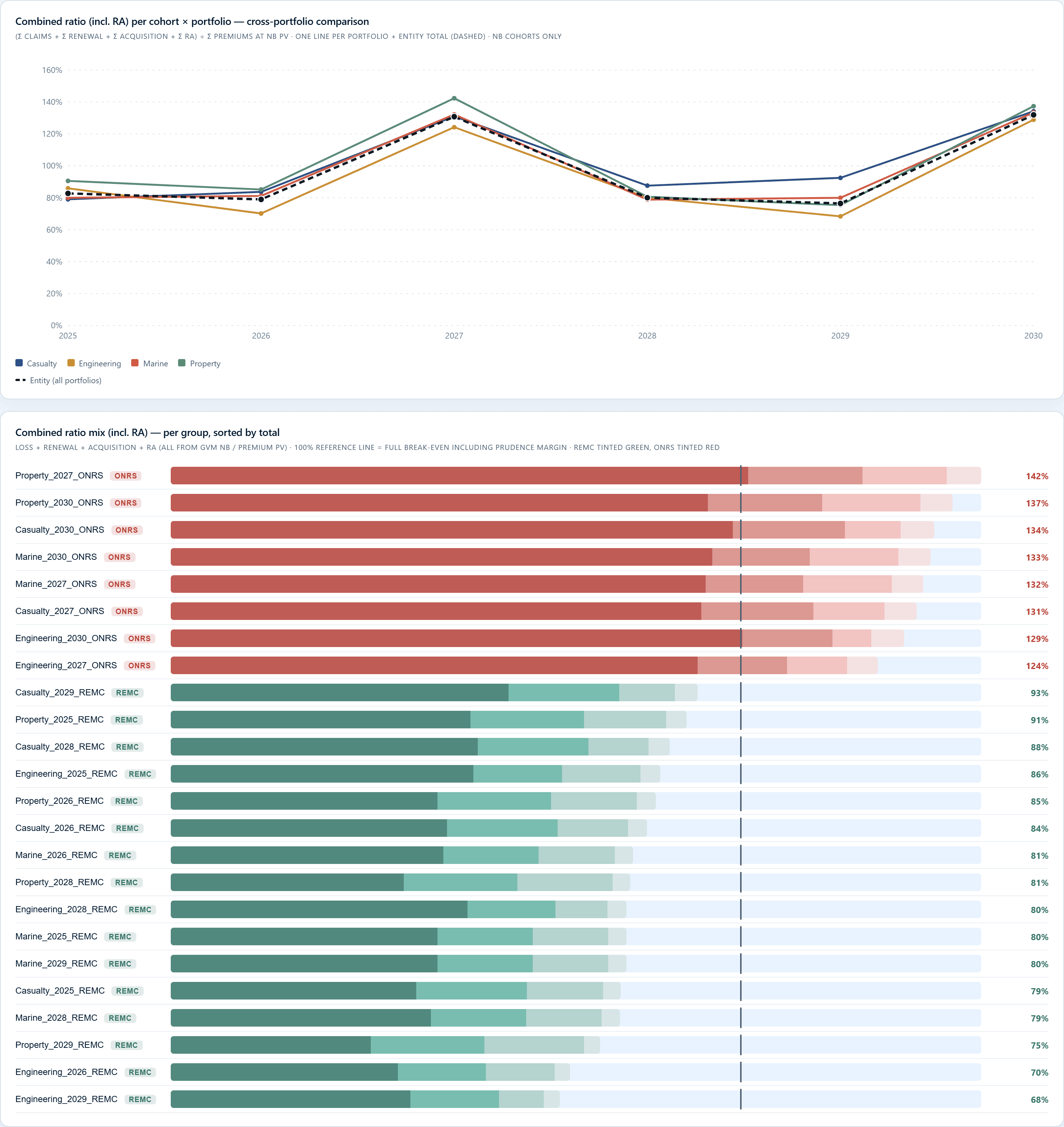
What this view catches: cohort-level lookup chains breaking; scenario shocks not propagating to the right cohort year; CSM release drifting from the chosen coverage-unit basis. A clean result across cohorts and scenarios is a strong indication the propagation from inputs to projections is intact.

View 2 — New business layering by cohort

A visualisation of the cohorts active at each future date, showing the age and the relative scale of each one.

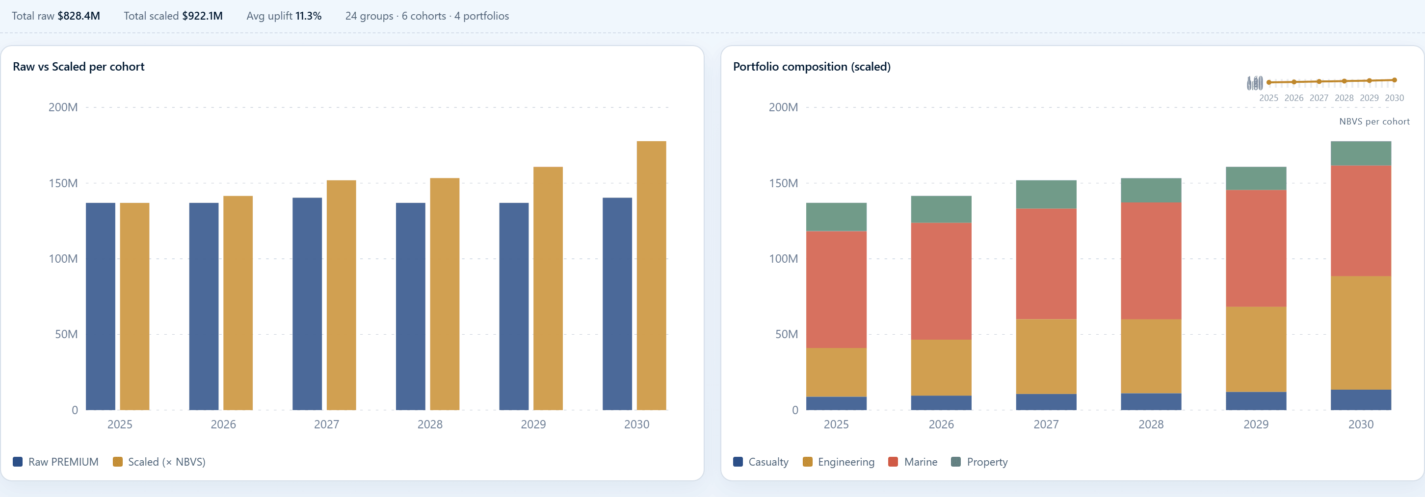
The first view to open in any forecast materially driven by future new business. Per-portfolio scalars should be visibly differential — Engineering compounding faster than Property — and the in-force cohort should appear once, not be re-recognised as year-1 new business.

View 3 — Measurement-component bridges (BEL, RA, CSM, LC, NDAC)

A waterfall for each measurement component — BEL, RA, CSM, Loss Component and NDAC — per year. The primary diagnostic for the GMM measurement layer.

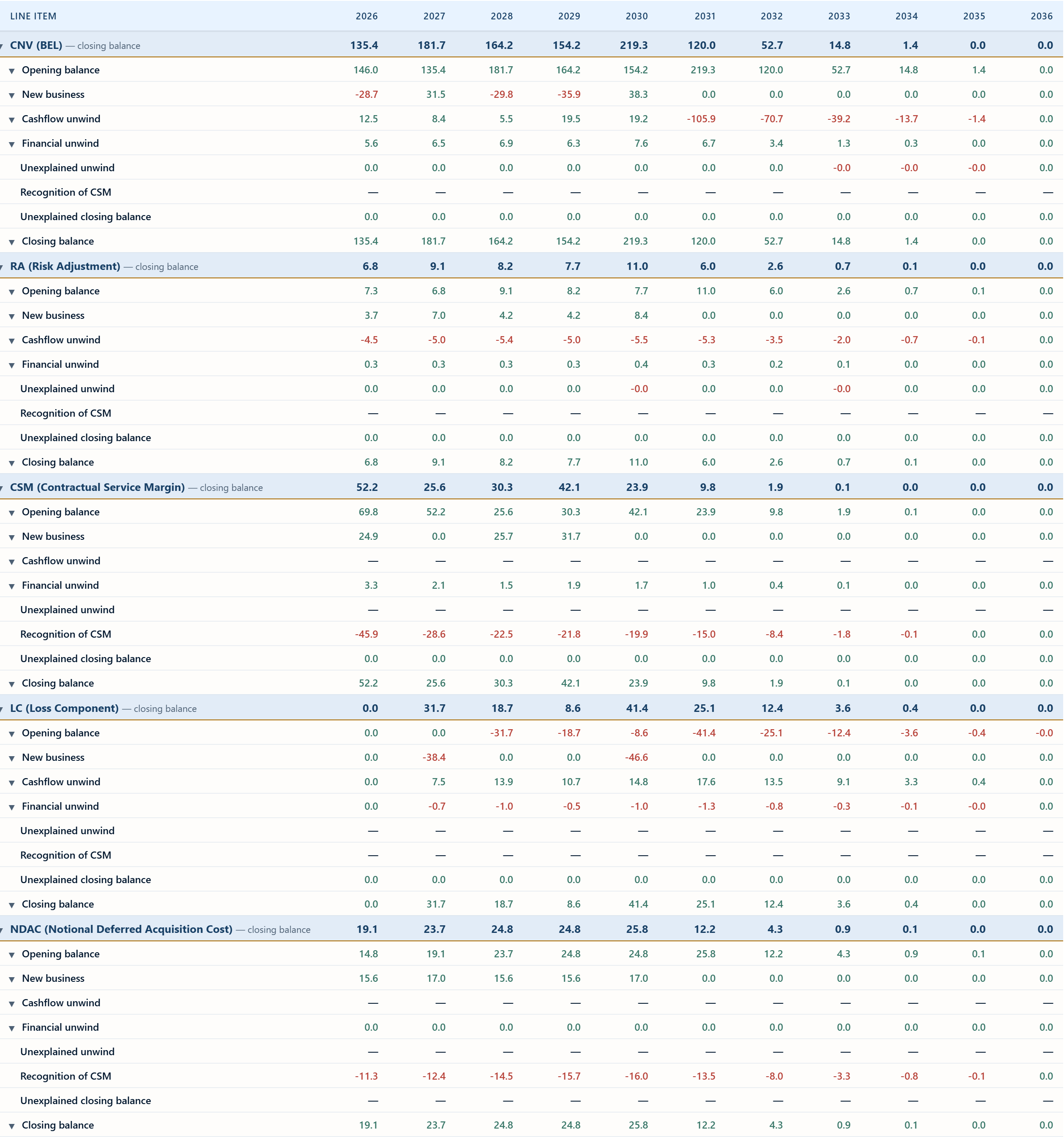
For each period the bridge shows opening, CSM unwind at locked-in rate, assumption-change adjustment, new business CSM, CSM release to revenue, closing. Where a group transitions state, the bridge shows the residual movement and the P&L posting explicitly.

What the bridge catches: a shocked cohort that should be onerous at initial recognition but isn’t; a loss component that is not releasing as the losses emerge; CSM unwind drifting from the locked-in curve (the rate is being re-derived rather than preserved).

View 4 — Per-group SOCI build-up

The income statement at the group level, with each of the IFRS 17 revenue components stacked: CSM release, RA release, expected insurance service expenses, NDAC amortisation, premium experience variance — the building blocks of insurance revenue under paragraph B120 — with the total insurance result overlaid.

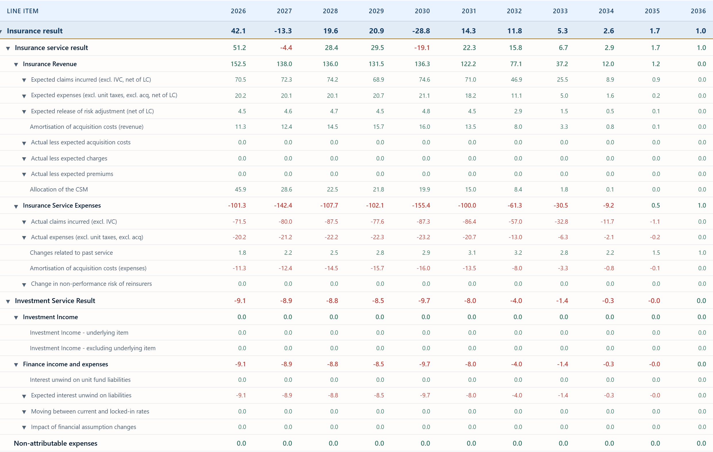
NDAC stands for Notional Deferred Acquisition Cost. Under IFRS 17 the acquisition expense is deferred notionally into the LRC measurement and released through insurance revenue (paragraphs 28 and B120) — it is not booked as a standalone Deferred Acquisition Cost asset as it was under IFRS 4. If you see NDAC sitting as a separate balance-sheet asset, the model is still under the IFRS 4 mental model.

This view also surfaces which group is doing the work. A profitable entity result can be one group with a large CSM release masking another with a quiet LC drag.

View 5 — Reinsurance loss-recovery component

A view that exists only because of GMM. When an LC arises on the underlying side, the ceded balance carries a loss-recovery component — LRC_Reinsurance = LC_covered × r. For proportional cover, r is the cession rate; for non-proportional cover, r is not the same as any single contractual ratio.

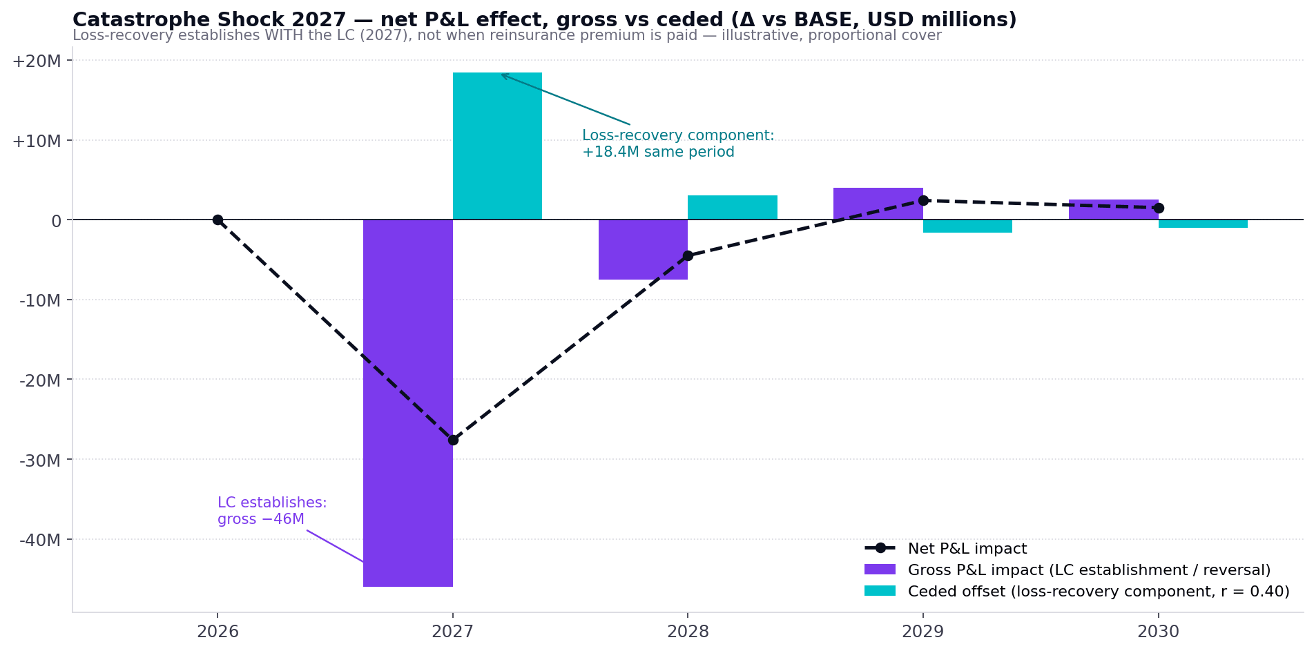
A PAA-style mirror that scales ceded revenue with premium volume will under-damp the net P&L impact of an onerous-group movement where significant cession is in place. Loss-recovery should establish when the LC establishes, not when reinsurance premium is paid.

View 6 — Debtor and creditor trajectory

The view that catches the actuals-inside-the-balance-sheet problem before it shows up as a CSM unlock you did not intend. The methodology requires two assumptions per future period for each flow type: the raised (or incurred) leg, supplied by the actuarial model, and the received (or paid) leg, which the actuarial model does not produce. Calibration is from recent financial-year actuals.

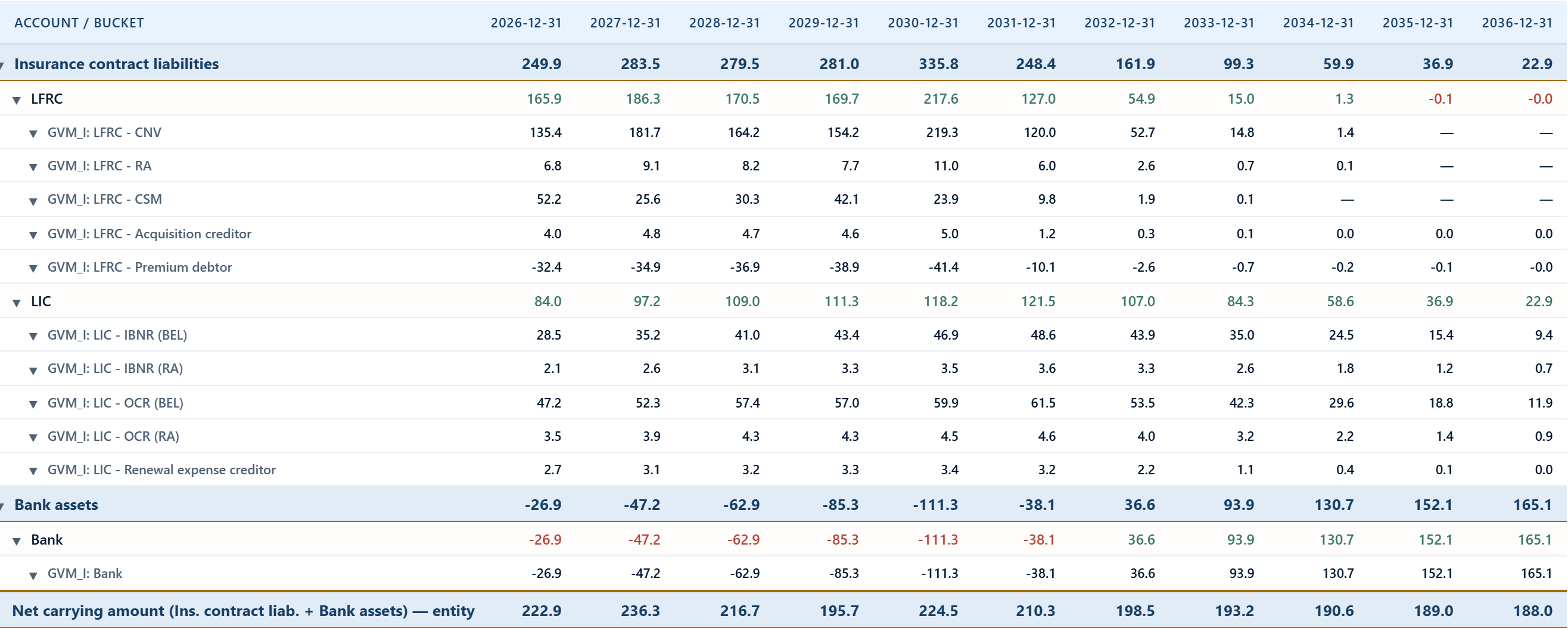
A debtor line flat across the horizon, against a growing book, flags under-specified accrual assumptions. Per-portfolio runoff matters: Casualty creditors hold longer than Property; if they all run off identically, the per-portfolio assumptions are tied together.

View 7 — Balance sheet by IFRS 17 group, net of reinsurance

The full group balance sheet stacked: BEL, RA, CSM or LC, LIC OCR, LIC IBNR, RA LIC, net of the reinsurance mirror. The view a board member opens when asking which group is carrying the liability and whether it is growing with the book.

View 8 — Bank trajectory

Cumulative bank balance year-end. If the bank goes negative, the book consumes cash faster than it generates it — possibly because claims pay before reinsurance recovers, or because acquisition spend front-loads. The dip is expected behaviour, and a useful planning input.

---

Why it ties out — the journal entries behind the views

A GMM forecast that ties out is a forecast built as a journal. Every BS movement has a Dr/Cr counterpart, and the closing balance is produced by the postings themselves.

Movement	Dr	Cr
BEL release of expected claims & expenses	BEL	Insurance Revenue (expected claims & expenses)
Premium cash-flow unwind	Premiums control account	BEL
BEL unwind on current rates	Insurance Finance Expense	BEL
CSM unwind on locked-in rates	Insurance Finance Expense	CSM
RA unwind on current rates	Insurance Finance Expense	RA LRC
LIC unwind on current rates (BEL and RA)	Insurance Finance Expense	LIC BEL / LIC RA
CSM release on coverage units	CSM	Insurance Revenue
RA release alongside risk emergence	RA LRC	Insurance Revenue
NDAC amortisation (paragraph B125 pairing, net nil)	ISE — acquisition amortisation	Insurance Revenue — acquisition recovery (paragraph B120)
LC absorbing day-1 loss on an onerous cohort	Insurance Service Expense — Onerous	LC
LC release as losses emerge	LC	Insurance Service Expense — LC unlock
Reinsurance loss-recovery component	RI asset — loss-recovery component	Insurance Service Expense — RI loss-recovery
Premium received	Bank	Premium Debtor
Expenses and acquisition costs paid	Expense / acquisition creditor	Bank
Claims paid — current service	Actual claims incurred (P&L)	Bank
Claims paid — past service	Changes related to past service (P&L)	Bank

Every movement is a double entry. Most pair the balance sheet with the P&L — CSM release ↔ Insurance Revenue, NDAC amortisation ↔ Insurance Revenue, LC absorbing onerous business ↔ Insurance Service Expense. The premium and expense cash legs are the exception: receipts and payments settle the debtor or creditor against bank, balance sheet to balance sheet. Claims paid post against bank with the P&L claims charge. Equity ties out in every period either way.

The insurance finance expense lines in that table — the BEL, CSM, RA and LIC unwinds — sit outside the insurance service result. IFRS 17 splits the result in two: an insurance service result (insurance revenue less insurance service expenses, the underwriting performance) and an insurance finance income or expense (the unwind of discount, which reflects the passage of time rather than service rendered). The total insurance result is the sum of the two. A forecast that folds the discount unwind into the service result overstates underwriting performance and understates the finance line; the projection should carry them as separate lines so the SOCI ties out the way the disclosure presents it. Where the insurer takes the OCI option for insurance finance income and expense (paragraphs 88–89), the unwind is split again between P&L and other comprehensive income, and the forecast has to route it the same way the accounting policy does.

A subtle point: aggregation matters. IFRS 17 paragraphs 16 and 22 require groups to be formed by portfolio, by issue cohort (the annual-cohort rule), and by profitability bucket at initial recognition. The standard does not permit free cross-subsidisation within a group — clearly-onerous contracts cannot be tucked into an otherwise-profitable group via aggregation. A forecast that aggregates new business onto the in-force cohort, or that mixes onerous and profitable measurement within a single group, produces a tied-out P&L that is not IFRS 17 compliant.

---

From view to engagement

If you are running an FY2026 GMM budget cycle — a life book, a long-tail non-life portfolio, or a reinsurance book — help building the views above, or a set of diagnostics built into the model from day one, sits within scope of the IFRS 17 forecasting work on this site.