Reading an IFRS 17 PAA forecast: the views that matter

FY2026 is the first full budget cycle most insurers and reinsurers are running on IFRS 17 baselines. The mechanics are different from IFRS 4 — earned premium replaces written premium as the headline; expenses split between attributable and non-attributable; reinsurance results sit on their own line; risk adjustment moves through P&L; and the balance sheet stops being a residual and starts being the spine of the result.

For reviewers — heads of actuarial, group reporting, audit committees, oncoming auditors — the lens shifts. A forecast that “looks right” against IFRS 4 muscle memory may be quietly broken under IFRS 17. The fix is to know which views to open first, and what each one is telling you.

This post walks through the ten views I look at when reviewing an IFRS 17 PAA forecast — four headline views that catch most issues, six supporting views for context and depth, plus the underlying mechanic that makes everything tie out.

The screenshots are anonymised but live — every chart in this post comes from a working PAA forecast model run over a multi-year monthly horizon. Portfolio names and currency labels are stripped; the magnitudes you see are real model output.

What a forecast actually does

Before the views, the framing. A forecast projects your insurance result forward, period by period, under a set of assumptions. It is how you:

• Test scenarios — claims shocks, growth slowdowns, ratio changes, reinsurance restructures
• Gauge trends — combined ratio direction, when it stabilises, where each line is heading
• See equity move — when surplus accumulates and when it erodes, and by how much
• Plan capital and solvency — project capital coverage forward, spot the period where it tightens
• Inform pricing and reinsurance design — set rate-change targets to hit a combined ratio, test cession structures before committing

A forecast that does only the first two of those is a chart. A forecast that does all five is a tool. The difference is whether reviewers can interrogate it from multiple angles and get coherent answers — which is exactly what the ten views below are designed to enable.

How a PAA forecast is built

Three pieces.

Inputs. Annual ratio assumptions per year × portfolio — claims, expense, acquisition, reinsurance ceded, recovery, commission, non-attributable expenses, growth, discount, runoff. Plus opening balances seeded from valuation-date actuals.

Mechanic. The first projection period is anchored directly to the seeds × the year-1 ratios. Subsequent periods roll forward via a monthly growth factor, then re-anchor to each year’s ratio assumption. Premium compounds; ratios self-correct each year to whatever you assumed for that year. This is what stops loss ratios from drifting.

Output. Projected P&L lines, balance-sheet roll-forwards (UPR, DAC, Premium Debtor, Creditor, LIC BEL, LIC RA), and bank — monthly, by portfolio, over the projection horizon.

The build is simple. The discipline is in how you check it.

---

View 1 — Implied vs assumed ratios

The first chart to open. Plot the implied ratios coming out of the projection — claims ÷ EP, expenses ÷ EP, acquisition ÷ EP — against what you assumed.

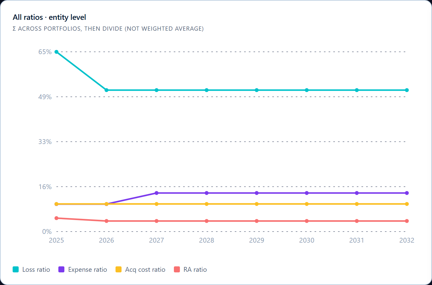
The chart above shows an OPEX +4pp shock scenario. The expense ratio steps up from ~10% to ~14% in 2027 — the shock landing exactly where the input changed. The claims ratio drops because the ratio recalibration logic resets at year-1; the unaffected ratios (acquisition cost, RA) sit smooth across the horizon.

What this view catches:

• Ratios that drift when they shouldn’t. If your claims ratio was supposed to stay flat but the implied line slopes, something in the roll-forward isn’t re-anchoring properly each year.
• Ratios that don’t move when they should. If you applied a shock in 2027 but the implied line is unchanged, your assumption isn’t propagating into the formula chain — most often a missing lookup, a hard-coded reference, or a variable that copies forward without re-applying the assumption.
• Magnitudes that are wrong. A loss ratio assumed at 65% but implying at 72% means either the formula is multiplying by the wrong base, or the ratio numerator includes lines you didn’t intend (PS releases, claims handling, RA flow).

If this view comes back clean, you’ve eliminated 80% of the formula-propagation bugs in one chart.

---

View 2 — Liability roll-forwards

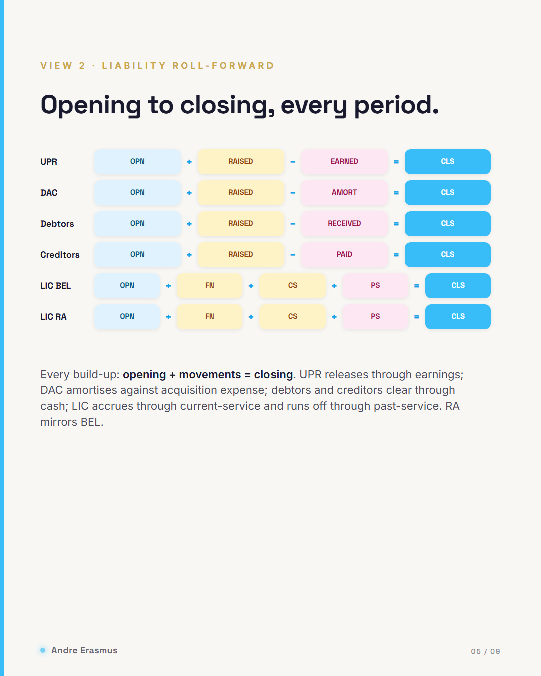
The balance sheet of a PAA model is six build-ups: UPR, DAC, Premium Debtor, Creditor, LIC BEL, LIC RA. Each follows a strict pattern:

Closing = Opening + Movements

For UPR: OPN + RAISED − EARNED = CLS (liability). New written premium adds to UPR; earned premium releases.

For DAC: OPN + RAISED − AMORT = CLS (asset). New acquisition cost defers; amortisation releases against P&L.

For Debtors and Creditors: OPN + RAISED − RECEIVED/PAID = CLS. The cash leg of premium and expense flows.

For LIC BEL: OPN + FN + CS + PS = CLS (liability). Opening claim reserve, plus discount unwind (FN), plus current-service accrual (CS) for new claims this period, plus past-service runoff (PS) for prior claims developing.

For LIC RA: same shape as BEL, scaled as a fixed proportion of BEL.

When stress-testing a model, the temptation is to look at each P&L line. The discipline is to look at each build-up. If a build-up doesn’t close, the P&L number that releases out of it is also wrong — even if it looks reasonable.

A second view to open after the cascades close is the net closing balance sheet by component — UPR, DAC, debtors, creditors, LIC BEL, LIC RA, all stacked year-end, net of insurance and reinsurance. You can see at a glance whether net liabilities are accumulating, when they peak, when they run off, and whether equity is building or eroding to fund them.

What to look for in that view:

• UPR and LIC BEL should grow with the book. If the book is growing and these liabilities are flat, something in the RAISED legs isn’t tracking premium volume.
• DAC should follow acquisition spend. If it spikes and decays unevenly, the DAC raised ratio probably isn’t being re-applied per year.
• Net result of insurance + reinsurance should be sensible. A given ceding rate should leave net liabilities in the expected proportion of gross. If R-side mirrors aren’t moving in lock-step, the reinsurance assumptions are decoupled from the insurance projection.

---

View 3 — Build-up checks

Every build-up has a closure test. The test is the same in every period:

Closing − Opening − Movements = 0

In a model built as a journal — every BS movement posted with its P&L counterpart — these checks are zero by construction. In a model built as parallel sheets that get reconciled at the end, they’re zero only when nothing has gone wrong, and you have to inspect them periodically.

Either way, the checks are a non-negotiable view. Nine of them across all periods is the floor:

• Check · UPR
• Check · DAC
• Check · Premium Debtor
• Check · Creditor
• Check · LIC BEL
• Check · LIC RA
• Check · Bank
• Check · R LIC BEL
• Check · R LIC RA

Each check returning 0.00 (within numerical tolerance, say 1e-6) across every period in every portfolio means the build-up is intact.

What these checks catch when they fail:

• Unposted movements. A new variable you added that moves the BS but didn’t get included in the closing formula.
• Sign errors. In the convention used here, assets are stored negative and liabilities positive; one sign flip breaks the cascade.
• Missing seeds. A t=0 opening balance that wasn’t loaded — the t=1 calculation picks up zero, the cascade collapses.
• Broken formula propagation. A roll-forward formula that references the wrong period or the wrong portfolio key.
• Currency drift. A scaling factor applied inconsistently across variables — the build-up still “balances” within the variable but the totals don’t reconcile across the rest of the model.

A model can produce coherent-looking P&L while one of its build-ups is silently broken. The check is the only way to catch it.

---

View 4 — P&L composition + Total

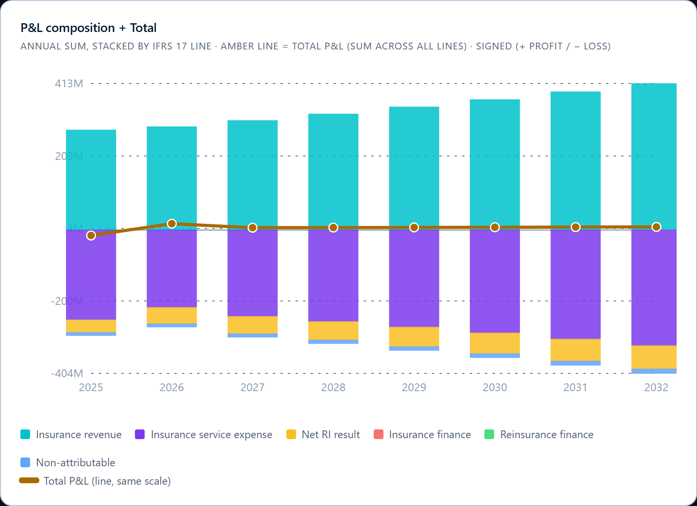
The headline result. Stacked annually by IFRS 17 line — Insurance Revenue, Insurance Service Expense, Net Reinsurance Result, Insurance Finance, Reinsurance Finance, Non-attributable — with the Total P&L overlaid as a line on the same y-axis.

This view answers four questions at once:

1. Where does profit come from? The visual stack tells you immediately whether revenue is growing faster than the expense bars, where reinsurance is helping or hurting, and whether non-attributable is a meaningful drag.
2. What’s the trajectory? The Total P&L line shows whether you are heading toward profit, away from it, or sitting flat. A line that stays close to zero across the horizon — as it does in the screenshot above — is a marginal book that needs price action or expense discipline to move.
3. Where do scenarios reshape the picture? Switch scenarios and the bars and the line move together. An OPEX +4pp shock pulls the Total P&L line down meaningfully and persistently — visible immediately, no spreadsheet diff required.
4. Are magnitudes plausible? Compare projected Insurance Revenue to last year’s actual. If you assumed 6% premium growth, year 1 should be roughly 6% above the prior period. If it’s 20%, you’ve double-counted growth somewhere.

What this view does not catch is composition issues that net out. A claims ratio that’s wrong by +5pp can be offset by an expense ratio wrong by −5pp and the P&L line will look fine. That’s why View 1 (implied vs assumed) sits ahead of this one in the review sequence — it catches the line-level errors before this view shows you their net effect.

---

Bonus views — the ones that don’t fit on a slide

The four views above will catch most issues. The next set of views are where depth comes from — context for board packs, anomaly detection, and the diagnostic detail needed when something looks off.

Earned premium projection

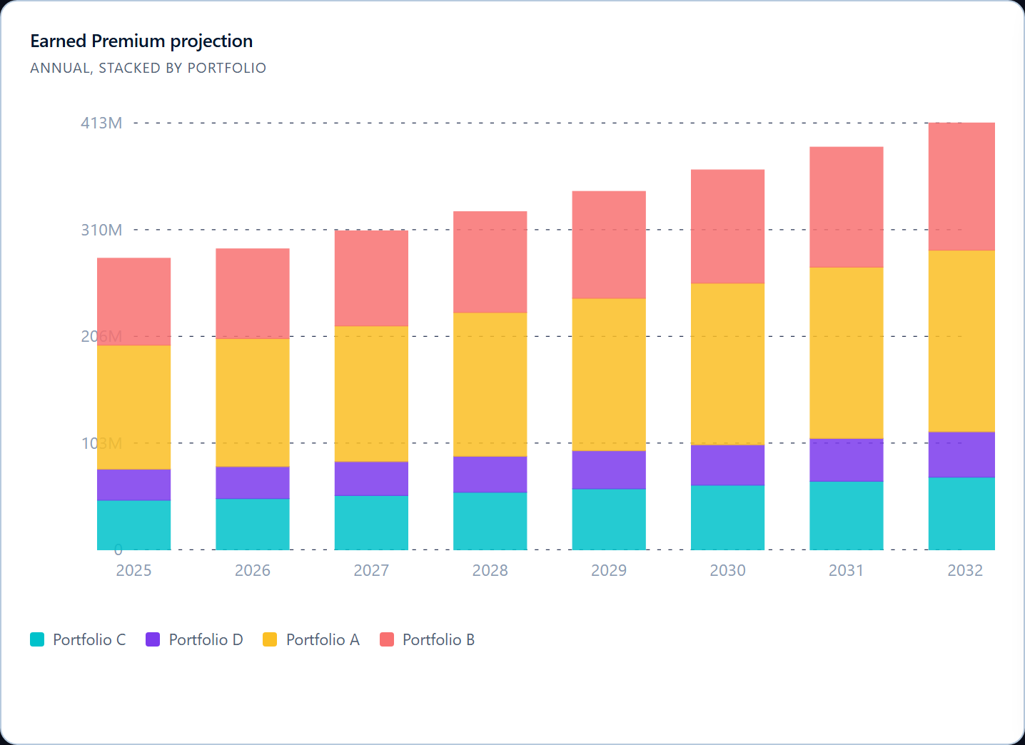
EP per portfolio over the horizon. Useful for sense-checking that growth assumptions are flowing through proportionately, and for spotting portfolios that are doing the heavy lifting (or dragging). When stressing a single portfolio’s loss ratio, this view shows the volume the stress is applied to.

Cumulative bank balance

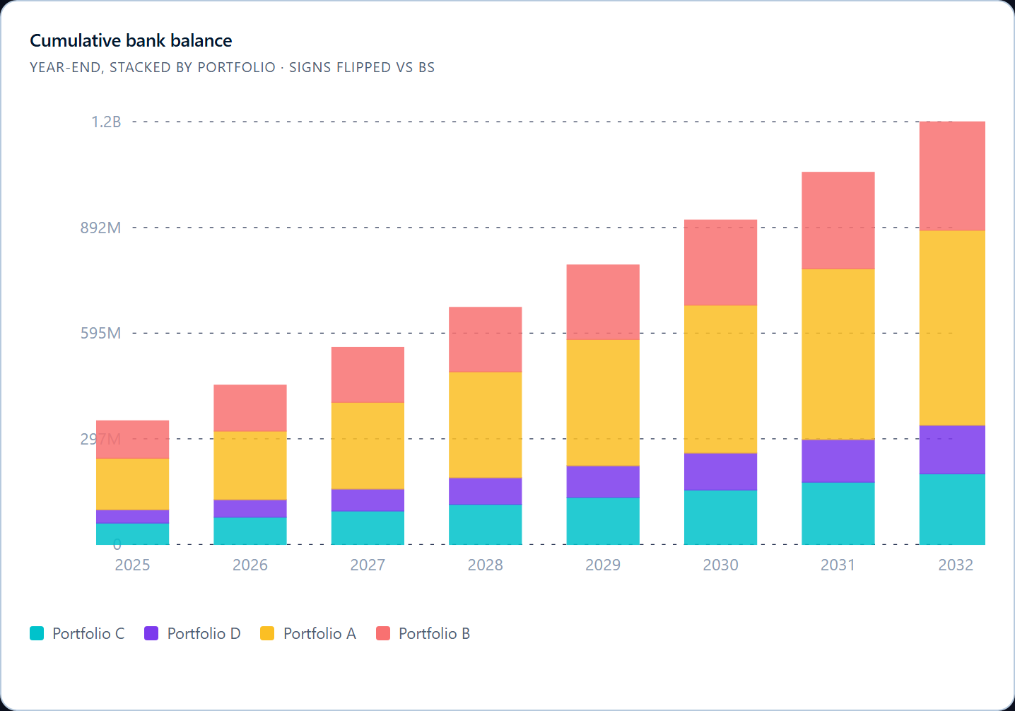
The cashflow story. Premium in, claims out, expenses out, RI premium out, RI recovery in, commission in. If the bank goes negative at any point in the projection, the model is telling you the book consumes cash faster than it generates it — possibly because claims pay before reinsurance recovers, or because acquisition spend front-loads. Either way, the dip is a planning conversation, not a model error. This is the view treasury cares about; it rarely flags a model bug, but it drives capital and liquidity decisions.

Loss ratio per portfolio

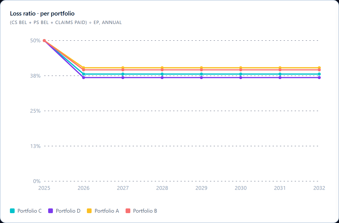
View 1 shows the entity-level implied ratios. This view splits them by portfolio. When the entity-level ratio is stable but the portfolio-level ratios are diverging, you know the mix is changing — one portfolio’s claims experience is pulling away from another’s, even if the average looks calm.

This is the view you pull up when a board member asks “which line is driving the result?”

Expense ratio per portfolio

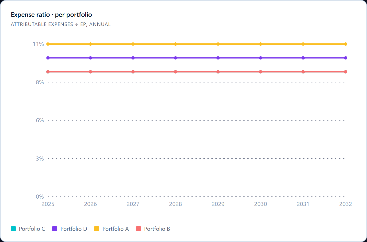
Same logic for attributable expenses. Useful for spotting portfolios where the expense load is structural (always high) versus cyclical (high in early years as the book builds, normalising as scale is reached).

Acquisition cost ratio per portfolio

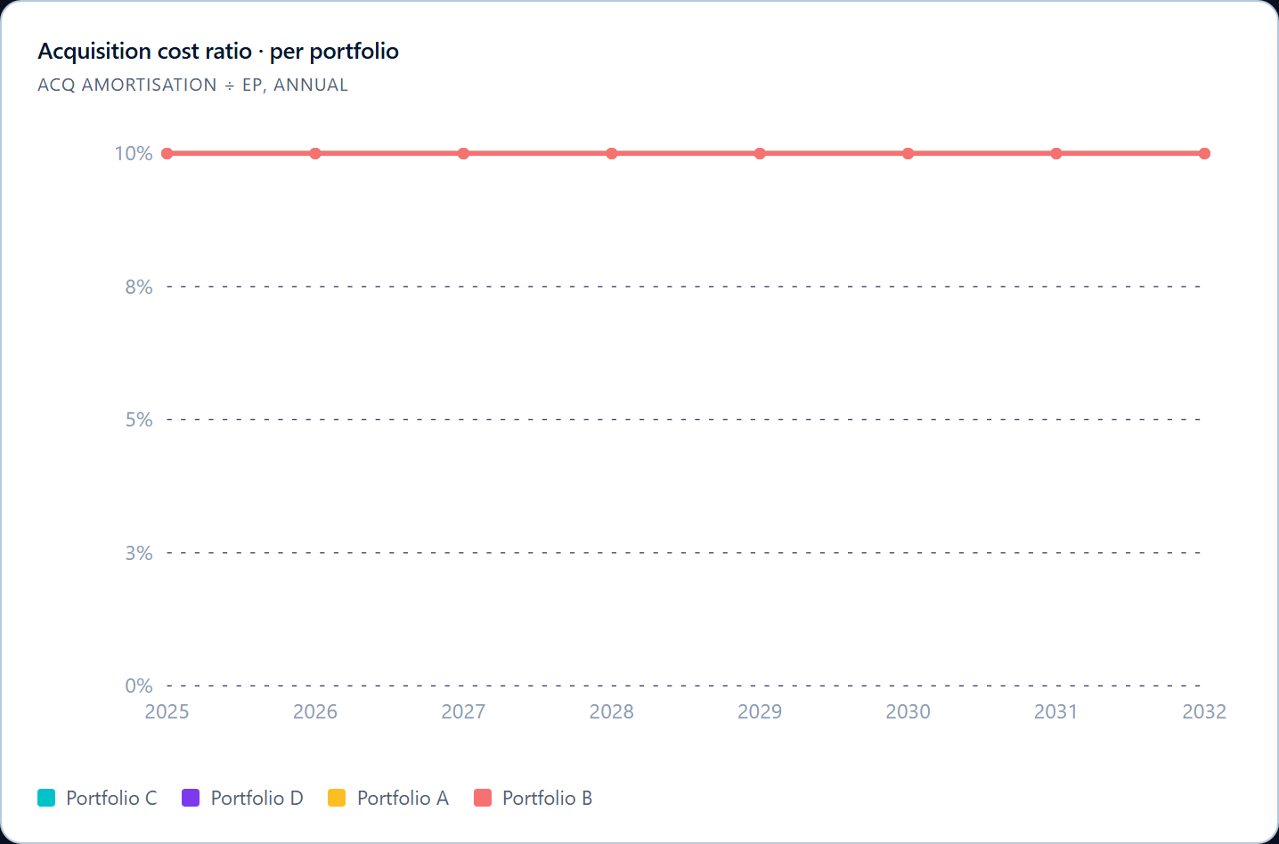
Acquisition spend as a fraction of EP. Two portfolios with similar headline acquisition cost can have very different ratios if they’re growing at different speeds — the ratio moves down as a portfolio matures, because EP catches up to the acquisition that drove it. Watch this view when discussing distribution strategy or commission structures.

RA ratio per portfolio

Risk adjustment as a fraction of EP. PAA models typically scale RA as a fixed proportion of LIC BEL, so this view is largely a function of the BEL trajectory. But if you set RA percentages by portfolio and they differ sharply, this view shows the relative risk loading you’re carrying.

EP-weighted input assumptions

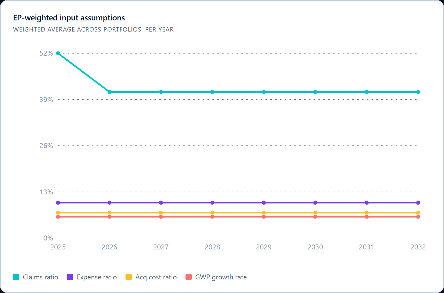
The closing diagnostic view. This shows your assumed ratios — claims, expense, acquisition, growth — weighted by EP across portfolios, plotted as the input side of the model.

Pair this with View 1 (implied ratios). If the implied lines and the assumed lines don’t track each other, the gap is what you need to investigate. If they track perfectly, your inputs are flowing through the model exactly as designed.

---

The six build-ups in detail

The four headline views and the six bonus views all rest on six build-ups. Each is a journal — every movement has a Dt and a Ct posting — so the closing balance is the result of the postings, not a calculated number.

UPR (Liability for Remaining Coverage — premium component)

UPR_OPN + UPR_RAISED − UPR_EARNED = UPR_CLS

UPR_RAISED is gross written premium for the period. UPR_EARNED is the amount released as Insurance Revenue this period. The release pattern under PAA is straight-line over coverage by default; non-uniform release is a Phase-2 extension.

DAC (Deferred Acquisition Cost)

DAC_OPN + DAC_RAISED − DAC_AMORT = DAC_CLS

DAC_RAISED is acquisition cost incurred this period (stored negative under the asset convention). DAC_AMORT is the portion released to P&L as Acquisition Expense. Under PAA, amortisation typically tracks UPR_EARNED, so the DAC release is proportional to the premium release.

Premium Debtor

Debtor_OPN + Debtor_RAISED − Debtor_RECEIVED = Debtor_CLS

Tracks the lag between premium written and premium collected. In Phase 1 of most builds, RAISED = RECEIVED — i.e., no lag, debtor stays at zero. In Phase 2, the debtor balance carries through and feeds the cashflow.

Creditor

Creditor_OPN + Creditor_RAISED − Creditor_PAID = Creditor_CLS

Mirror logic for outflows — acquisition payable, expense payable, claims handling payable. Same Phase-1 simplification: usually paid = incurred at outset, expanded in Phase 2.

LIC BEL (Liability for Incurred Claims — best estimate)

LIC_BEL_OPN + LIC_BEL_FN + LIC_BEL_CS + LIC_BEL_PS = LIC_BEL_CLS

Four movements:

• FN (Finance / unwind) — the discount unwind on the opening balance. Equal to discount_rate × OPN per period.
• CS (Current Service) — the new claims accrual for the period. Sized by claims ratio × earned premium, then split by the historical t=0 mix between cash paid and BEL accrual.
• PS (Past Service) — runoff of the opening claim reserve. Controlled by PS_runoff_annual; e.g., 50% per year leaves ~25% outstanding after two years.
• Closing — the sum.

LIC BEL is the most analytically interesting build-up. It captures both new claim emergence and prior-claim development, and the PS runoff parameter is one of the dials a sensitivity analysis turns first.

LIC RA (Liability for Incurred Claims — risk adjustment)

LIC_RA_OPN + LIC_RA_FN + LIC_RA_CS + LIC_RA_PS = LIC_RA_CLS

Same shape as BEL, scaled as a fixed proportion of BEL via a single parameter (RA_PERCENTAGE = RA_OPN / BEL_OPN). The RA release through P&L follows BEL release proportionally.

---

Why it ties out — the journal mechanic

The model is a journal, not a spreadsheet. Every variable is a posting with an explicit debit and credit:

Movement	Dt account	Ct account
UPR_RAISED	Premium debtor	UPR
UPR_EARNED	UPR	Insurance Revenue
DAC_RAISED	DAC	Cash — or Acquisition Creditor in models with a cash lag
DAC_AMORT	Acquisition Expense	DAC
LIC_BEL_FN	Insurance Finance Expense	LIC BEL
LIC_BEL_CS	Insurance Service Expense — Claims CS	LIC BEL
LIC_BEL_PS	Insurance Service Expense — Claims PS	LIC BEL
LIC_RA_*	parallel into RA accounts	LIC RA
Cash claims paid	Claims Paid	Cash

Every BS movement has a P&L counterpart, by construction. UPR EARNED ↔ Insurance Revenue. DAC AMORT ↔ Acquisition Expense. LIC CS ↔ Claims Expense. There is no “manual reconciliation step” between the BS and the P&L — equity ties out in every period because nothing moves on the BS without its mirror moving in the P&L.

This is the structural reason View 3 (build-up checks) returns zero. If you build a forecast as parallel BS and P&L sheets and reconcile them at the end, the checks return whatever residual the spreadsheet happens to have. If you build it as a journal, the checks are zero by construction — the Closing balance is defined as Opening + Movements, and the Movements are defined as the same numbers that flowed into the P&L.

The practical implication: a PAA forecast that is hard to reconcile is a PAA forecast built on the wrong substrate. Move it to a journal-style model, and the reconciliation problem dissolves.

---

Preview — scenario testing

The four headline views and the six bonus views are the BASE-scenario diagnostics. Once they are clean, scenarios are where the analytical value sits.

A scenario in this context is a coherent set of input changes — a claims ratio bumped by 5 percentage points across all portfolios, an expense ratio hit with a +4pp OPEX shock, a 2027 recession that simultaneously slows growth and drives loss ratios up. Each scenario is a self-contained set of assumptions; the model re-projects under those inputs and produces the same ten views, in the same shapes, with different numbers.

The chart at the top of this post — the implied ratios under an OPEX +4pp shock — is one such scenario. The expense ratio jumps where the input lands. The claims ratio drops because the ratio recalibration moves with the new period-1 anchor. Other ratios stay flat.

The next iteration of this post will show side-by-side comparisons under three scenarios — claims +5pp, OPEX +4pp, and a 2027 recession — across all ten views. Same model, same horizon, three different futures, and the points where they diverge are where the planning conversation actually starts.

---

From view to engagement

If you are running an FY2026 PAA budget cycle, a second pair of eyes on the views above — or a reviewer-ready set of diagnostics built into the model from day one — sits within scope of the forecasting services and software work on this site.